Convergence of Solution in Scientific Programming

Introduction

For most of the computational problems that are solved using programming, the objective is to find problem solution(s) using a suitable numerical method. This is because, either there hardly exists an analytical solution for such problems or the feasibility of computer implementation of such (analytical) solution(s) is extremely low. Most of the times, the exact numerical answer of the problem is unknown. In such a case, the question is how to get most accurate numerical value of solution for the problem under investigation? Though there is not any straightforward answer to this question, still it is worth to discuss few things in this regard. Basically, this question has two different perspectives.

The first one is that, most of the numerical methods are iterative in nature which means in successive steps, we approach closer and closer towards exact solution which most of the times is unknown. Therefore, the number of iterations that should be performed for getting exact solution is not known in advance. Further, we cannot simulate extremely large number of iterations as it will incur extremely high computational burden which is of course is not encouraging.

The second thing is that, if the accuracy of solution is increased in successive iterations, then at what accuracy level (% error value) we should stop our calculations? Because there is a limit on identification of small values by our computer system. In our earlier post, we have discussed about it.

It is not surprising that, as the solution becomes more and more accurate in successive iterations, the rate of decrease of error (gain in accuracy) also diminishes and this change is noticeable.

Consider a very simple example of finding value of π by calculating the perimeter of circle by approximating its value with the perimeter of an inscribed polygon inside the circle. We can see that, as the number of sides of polygon increases, we get more and more precise approximations of circumference of circle. (A circle can be assumed as a polygon of infinite sides.) However, we simply can’t inscribe a polygon of infinite sides inside any circle. Hence our polygon will have finite number of sides say N.

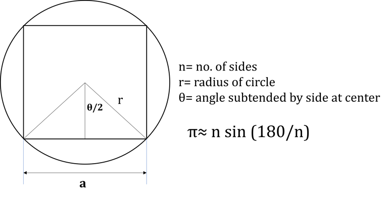
Secondly, imagine that you don’t know the value of π. Then in this case, at what value of N, the value of π so obtained by this method can be considered good enough.

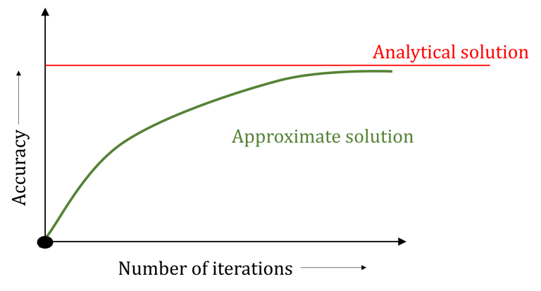
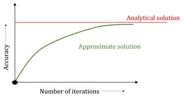
If we plot a graph of number of sides of polygon against accuracy of solution, we will see that, we get a curve as shown in figure.

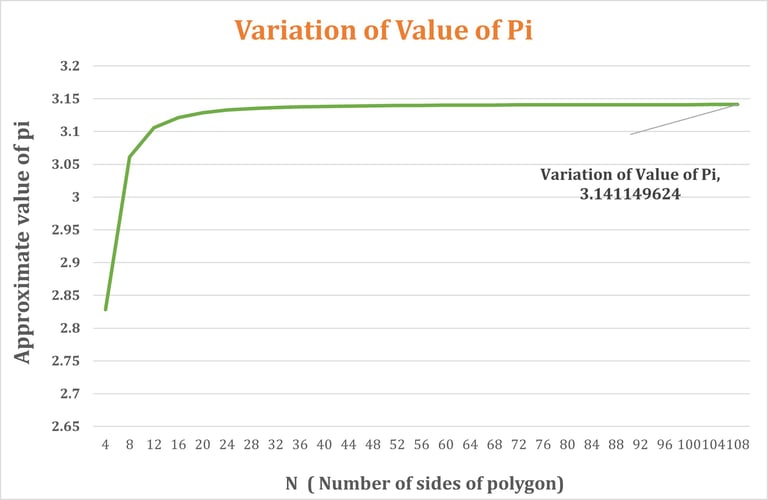
Same is the nature of curve that we get for iterative algorithms (provided that the method we are adopting ensures convergence.)

One wise approach to stop iterations is to compare the solution (S) obtained in n+1th iteration with that obtained in nth iteration and calculate the change e such that e = (Sn+1-Sn) (Note that the term Sn+1-Sn indicates improvement in accuracy of solution in n+1th iteration)

As algorithm proceeds, e becomes smaller and smaller. The smallest value of e that can be identified by our computer system is machine epsilon and it is generally denoted by eps. Therefore, one of the criteria for stopping computations is e<=eps.

But this is not a requirement always. Let’s demonstrate an example of finding fifth root of 27 using Newton- Raphson method. This is as good as solving the following equation.

X^5-27=0

If you are familiar with excel VBA, then copy following VBA code. Open MS excel, go to developer mode and paste it inside visual basic editor and click run macro.

Option Explicit

'The Newton-Raphson method for finding fifth root of 27

Sub NR()

On Error Resume Next

'Formatting commands start (these are optional)

ActiveSheet.Range("A1:B13").WrapText = True

Columns("A").ColumnWidth = 10

Columns("B").ColumnWidth = 15

Range("A2:B1000").Clear

'Formatting commands end

Dim start As Double

Dim R As Range

Dim x_new As Double

' program to find 5th root of 27

Dim i As Integer

Dim x_old As Double

start = Application.InputBox("Please enter the initial approximation", "User Input")

Set R = Range("A1:B1")

x_old = start

R = Array("Iteration count", "Successive Approximations")

For i = 1 To 1000

x_new = x_old - (f(x_old) / fn(x_old))

Cells(i + 1, 1) = i

Cells(i + 1, 2) = x_new

If Abs((x_new - x_old)) <= 0.000001 Then

Exit For

End If

x_old = x_new

Next i

End Sub

Function f(x_old As Double) As Double

f = (x_old ^ 5) - 27

End Function

Function fn(x_old As Double) As Double

fn = (x_old ^ 4) * 5

End Function

If you are not familiar with VBA, then you can download this macro enabled workbook from here.

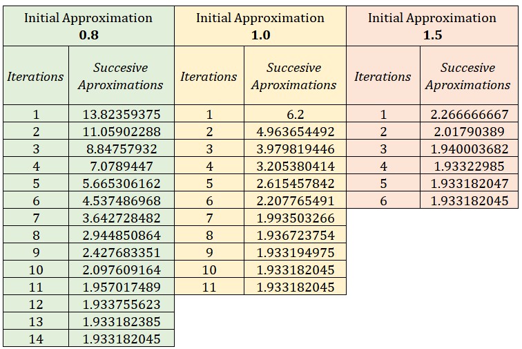
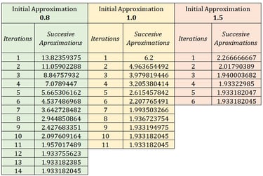
The results of program for initial value of 0.8, 1.0 and 1.5 are given below. The interesting fact here is that, the solution stopping criterion used in above program is |Sn+1-Sn|<= 0.000001.

Instead, we can also define solution stopping criterion as |Sn+1-Sn|<= e as discussed above.

Final thought

At this moment of time, you might be thinking that, how to ensure convergence of solution when applying a computer oriented numerical technique to the problem. Well, as mentioned earlier, though the answer to this problem is not straightforward, still one should keep following two things in mind.

1. Scientific programming is just a tool and not solution itself. Therefore, while dealing with the numerical problem, what actually matters is the acceptable accuracy or acceptable error in the solution. Which further depends on the nature of application under consideration. E.g. an application of simulating navigation of driverless automated guided vehicle requires very high precision when compared with precision required in the problem of modelling a counter weight for an electrical hoist (due to high factor of safety in its design considerations.)

2. Before applying computer programming to a numerical method, one should be aware of its pros and cons and should know the underlaying theory of its working.

Leave a reply