Scope of Scientific Computing

Scientific computing involves systematic use of computers in implementation of mathematical techniques towards solving complex engineering and real-world problems from various domains. At first glance, this definition of scientific computing appears very straight forward. However the scope of scientific computing is not just limited to finding solution of complex engineering or real-world problems, it is also a powerful tool used in mathematical formulation of the problem itself.

Scientific computing is widely applicable in following areas

1. Finding analytical (exact) solution of problems where exact mathematical model is available.

2. Finding numerical (approximate) solution of problems where exact mathematical model is available.

3. Finding numerical solution of problems where the mathematical models are somewhat approximate (e.g. probabilistic models.)

4. Problems where large numbers of governing variables are involved which makes analytical framing of mathematical model extremely difficult. Such problems demand vast experimentation and identification of pattern of experimental data obtained thereafter.

5. Optimization problems. (usually involve selecting unique solution from different available choices.)

6. Problems involving graphical representation of complex scientific data.

7. Machine learning problems.

Obtaining solution for an engineering / real-world problem mainly involves following steps.

1. Observe the phenomenon/system.

2. Identify and enlist the variables affecting the phenomenon/system.

3. Perform experimentation with system under study (generate the experimental data.)

4. Using principles of mathematics, known laws of physics and nature, certain governing principles, establish a mathematical relationship between variables affecting the physical phenomenon i.e. generate a mathematical model.

5. Validating the above relationship by preforming further experimentation i.e. validation of derived mathematical model.

Let us try to understand these problems with simple real-world examples.

Consider the example of Fourier law of conduction.

Mathematically it is described by equation

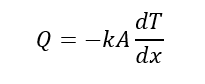
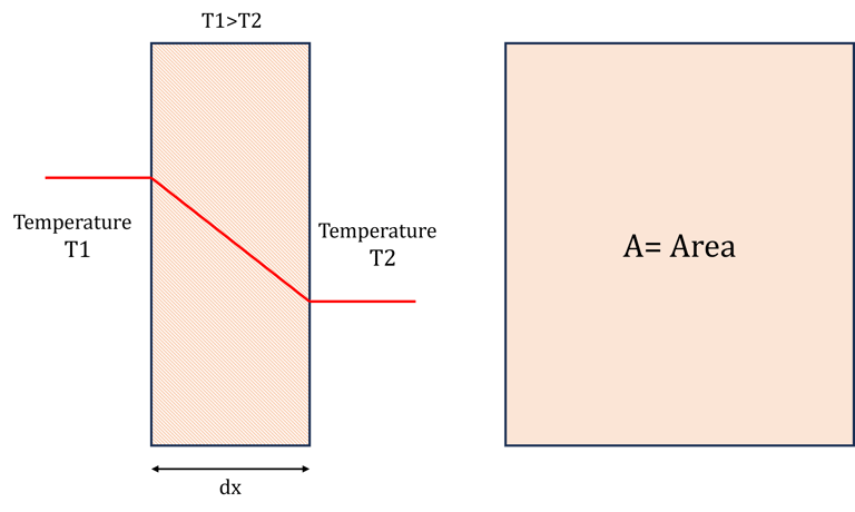
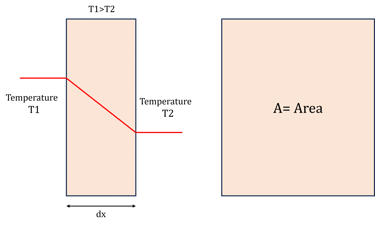
Long back in the history when this equation was not ready, scientist observed that the heat transfer rate through an object (say brick) changes when a temperature difference across the object was changed. Further it was discovered that any change in the thickness of object affected the heat transfer rate. In addition, they also discovered that heat transfer rate was affected when area of object was altered.

A Series of experiments were performed to estimate the effect of

• change in length of object (x) on heat transfer rate (Q)

• change in area of object (A) on heat transfer rate (Q)

• change in temperature difference at object ends (T1-T2) on heat transfer rate (Q)

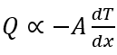
Data generated from these experiments revealed that

• Q was in direct proportion with A

• Q was in direct proportion with (T1-T2)

• Q was in inverse proportion with (x)

Thus, following relationship they obtained.

Minus sign shows decrease in temperature with increase in length

Further, it was discovered that when material of object was changed, the value of Q also changed even if the all-other physical aspects of the experiment remain the same. Subsequent experiments on objects of different materials led to the discovery of k (The unique property of material called thermal conductivity.) which is nothing but a constant of proportionality in above equation.

Here both exact mathematical model and exact solution are available. Need of computers to solve such problems is mainly due to vast and repetitive calculations usually involved in obtaining solution.

To understand this, consider a problem of a thick plate of variable (temperature dependent) thermal conductivity where one end of plate is exposed to hot gases and another end is open to atmosphere. If we want to plot a smooth temperature gradient across the plate. It requires calculating temperature values over different closely spaced points (say 50 or 100 points) across the length of brick. Here the task is repetitive in nature. Moreover, calculations tend to increase with increase in number of points. Solution to this problem can be automated with help of computer simply by using a spreadsheet program like MS excel. This is a very basic level of scientific computing.

This problem belongs to first category

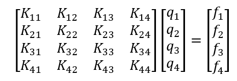
Consider the example of bending of a beam with governing equation given by.

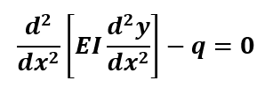
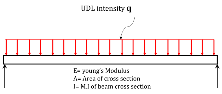
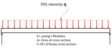
Using finite element method which we will be covering later in detail on this platform, we can reduce above differential equation into set of algebraic equations as given below

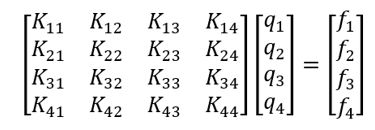
Well, you might be thinking that, the above differential equation is quite easy to solve an there is no need to convert differential equation into set of simultaneous linear equations. But in practice, the governing differential equations which exactly represent real-life problems may be extremely complicated to such an extent, that it is almost impossible to solve them analytically (recall Navier-Stokes equations.) The only choice to address them is the use of numerical methods like FEM, FDM, FVM etc.

The size of matrix in above example depends upon number of nodes which in turn depends upon level of discretization for a given problem. For example, if we divide our beam into two elements, the size of K matrix will change from 4×4 to 6×6. For 3 elements, it will be of 8×8 and so on. A real-world complex scenario can include dividing a given complex problem into include several thousands of elements generating matrices of dimensions several thousands. Thus demanding a powerful computer and a robust scientific programming method to solve it.

Such problems belong to second category

Consider the example of busy clinic’s appointment scheduling problem.

Here, the problem is to schedule the appointment of patient with doctor. The patient arrives at clinic counter and enrolls his name with required details. The receptionist feeds the patient data in clinic’s software and software estimates the approximate waiting time for patient. Further, next patient arrives and this process goes on. The computations of waiting time are based on queuing model known as M/M/1 Model. Framing this queuing model requires past data like

1.  Patient arrival rate

2. Service rate

3. Number of counters

4. Queue discipline (e.g. First patient first as in this case)

5. And capacity of system.

Based on this past data, a queuing model is generated. The interesting fact here to be noted is that this model is probabilistic in nature which means it is not exact.

This problem belongs to third category

Consider the following example.

In a survey conducted with the help of tyre resellers, the average wear percentage of tires of popular brands fitted to newly purchased cars of same segment and running as taxies was noted against the odometer reading (kM.) A cluster of these readings is obtained as shown in figure. With the help of this cluster, it is possible to predict the average percentage wear on tires for a given running distance for any new tyre purchase. This is a problem of regression. As seen from the figure, the best fit entity which represents the pattern of cluster is a line here. Thus, this is a problem of linear regression.

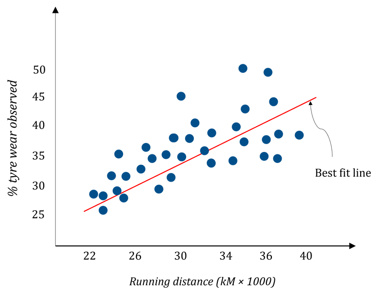
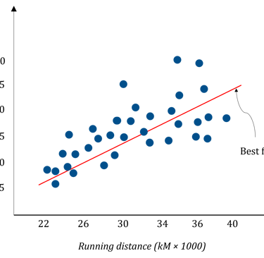
Usually, the data involved in surveys is enormous and it requires programming to address these types of problems. This problem is an example of single variate regression where there is one single independent variable and single dependent variable which is generally not a real world scenario. It is obvious that the life of tyre depends on many other factors like road conditions, driving habits. A multivariate regression problem is best suited for this. The problem of predicting loan default probability (LDP) of a customer based on his credit score, income, and tax payment history is  another example of multivariate regression.

These problems belong to fourth category.

Consider a problem of designing a combustion engine with the goal of maximizing fuel economy and minimizing harmful emissions like HC, CO and NOx

In this problem, the variables affecting combustion chemistry are

1. Injection timing,

2. Valve timing

3. Relative air fuel ratio, and

4. Engineering design of combustion chamber.

These factors also affect engine performance especially power and torque of engine and knock / detonation phenomenon.

The problem here is to decide optimum engine setting which involves obtaining the values for above variables such thatthey will

1. Reduce knocking/ detonation tenancy of engine over operating range.

2. Maintain a required torque-speed characteristics of engine over operating range and

3. Ensure delivery of rated power at specified crankshaft rpm.

And these are the constraints for engine designer.

It is to be noted that the effects of most of the variables listed above on engine performance are well known. But still, we cannot obtain analytical solution to this problem due to

1. Involvement of number of variables

2. Presence of multiple constraints for design engineer.

Such problem needs advanced engine cycle simulation techniques and chemical kinetics modeling software. Fortunately, a handful of scientific computing tools are available for dealing with such problems.

This problem belongs to fifth category.

Consider the problem where we want to visualize the temperature distribution in a plate which is given by

Where, (x, y) are the coordinates of a given point

The figure below shows visualization of the temperature distribution inside the plate with the help of Scilab.

The code to generate this temperature distribution is given below.

clc

clear

clf()

x=linspace(-75,75,150) // Generates 150 linearly spaced points between limits -75 to +75 in X dimension

y=linspace(-75,75,150) // Generates 150 linearly spaced points between limits -75 to +75 in Y dimension

function T=temperature(x, y)

T=y^2-16*x // Defines the given temperature function

endfunction

Sfgrayplot(x,y,temperature) // Use of Sfgrayplot function

gcf().color_map=jetcolormap(16) // Uses 16 colour shades between blue and red to generate contours

colorbar(283,1083) //displays a colour scale between 283 to 1083 which are minimum and maximum values on the plot respectively

xtitle("$\LARGE Temperature..Distribution $")

This problem belongs to sixth category.

Machine learning problems

The problems so far, we discussed above requires explicit programming or use of scientific tools for case. e.g. consider a scenario of family of problems involving calculation of strengths of different structural member under the action of three-dimensional loading. These problems can either be solved with the help of any standard FEA package or using a python programing with finite element method. Each of these approaches has its own advantages and disadvantages. Still one thing that is common in both of these methods is that, for every individual case, it requires programing and custom settings of options (in the case of if a standard FEA package is to be used.)

Machine learning (ML) is a science that enables computers to learn from dataset and further it can make decisions/predictions without being explicitly programmed for every single task. It involves training a system from past / historical data. Once system is trained, it becomes capable of recognizing patterns from existing data. These ML powered systems are capable of adapting and improving over the time —just like humans explore heuristic knowledge. Thus, eliminating the need of explicit programming for every new task.

The problems those are solved by Machine Learning algorithms fall in seventh category

Leave a reply