Finite Element Method- A Powerful Numerical Computing Method

Introduction to FEM

Finite element method is a powerful numerical methos to solve complex engineering problems which are either difficult or rather impossible to solve by analytical methods available with us. The method finds extensive applications in the various engineering fields including but not limited to applications involving stress analysis, heat transfer analysis, fluid flow problems, magnetic flux, acoustics and dynamic analysis problems. The real potential of this method came into picture after the advancements in computer technology and revolution in fast operating modern age processors. Today several FEA packages like ANSYS® COMSOL® LS-DYNA® are commercially available which are based on this method. With the advancement in computer graphics, various CAD models of a part can be developed within considerably small time period and they can be analyzed using FEA software which gives reasonably accurate predictions about the behavior these parts before their actual prototypes are built for testing. This saves considerable cost and time in product development. The unique future of this method is that it is highly systematic in nature which makes its computer implementation very easy. The method involves discretizing the domain under investigation into number of simpler subdomains also called finite elements. The behavior of filed variable which is also the basic unknown in the problem (like displacement in the problem of stress analysis and temperature in the problem of heat transfer analysis) is expressed in terms of its nodal values and is interpolated over an element using some suitable interpolation function. From the given data e.g., geometry and material the element level equations are formulated. These element level equations are further used to build the global equations i.e., the equations which are valid for entire domain. After incorporating appropriate boundary conditions, the system of equations is solved to obtain values of field variable at nodal points. From these nodal values of field variables, all other derived quantities of interest are calculated.

Basic Idea of finite element method

Engineering problems like stress analysis, heat transfer analysis and fluid mechanics involves some basic unknows like displacement, temperature, and velocities respectively. For a given domain, these unknows can take infinite values. For example, consider a solid mechanics problem of a bar fixed at one end and subjected to a pull at another end, the bar will undergo deformation. Now there are infinite points between the two ends of bar and at each point, there will be some value of displacement. Thus, the displacement can take infinite values as we move from fixed end to another end of bar. Finite element method converts this infinite displacement problem into finite displacement problem by dividing the entire domain (the bar in this case) into number of finite elements (subdomains). Now the unknown filed variables are expressed in terms of their nodal values (values that these filed variable assumes at nodal point) with the help of some interpolating functions also called shape functions. These shape functions actually describe the variation of these field variables over an element. Now the infinite unknowns in our original problem are reduced to finite numbers i.e., unknows at nodal points. Next, we define the element level equations using the data of problem. In this example the element level equations are force-displacement relations valid for an element.

 [ke][ẟe] = [Fe] -----(1.1)

Where,

• [ke] = is a matrix which establishes the relation between force(s) and displacements

• [ẟe] = vector containing nodal values of field variables (displacements at nodes in this case)

• [Fe] = vector containing the forces acting on the element

Equation 1.1 is valid for an element and therefore suffix e is used to denote the same.

Now, using systematic assembly process, the element level equations for each individual element are combined to write force displacement relations for entire domain. If suppose there are n elements in a problem, the n elemental equations will participate in formulation of domain level equation

 [K][ẟ] = [F] -----(1.2)

Equation 1.2 is valid for an entire domain. And matrix [K] is called global stiffness matrix. The term global symbolizes the meaning of validity over entire domain. Further by incorporating suitable boundary conditions as specified in problem, the system of simultaneous equations given by equation 1.2 is solved to find nodal values of field variables (entries in [ẟ] vector). Having found the nodal unknowns, the value of field variable at any non-nodal location within an element can be obtained by using the shape functions which shows the variation of these field variables over an element as stated earlier. It is interesting to note that all other derived quantities like stresses in solid mechanics problems and heat transfer rates in heat transfer analysis problems can be systematically found from these values of field variables by using certain relationships and governing laws.

Another interesting fact in above discussion is that, the original problem of a bar fixed at one end and subjected to a pull at another end can be represented by a differential equation of second order where the dependent variable of interest is displacement. The analytical methods involve solving these differential equations. Sometimes it is easy to solve such governing differential equations which captures physics of the problem especially when the problem is simple and not much complexities are present in problem as in above case. However, if given problem involves complexities in terms of material, geometries and loading, solution of the governing differential equation becomes difficult or rather impossible at times. If we look at equation 1.2, it represents, the system of simultaneous equations which are algebraic in nature. Therefore, it is much easy to solve it as compared to solving a complex differential equation. Now one may question that, what if the size of matrices is extremely large i.e., these algebraic equations are more in number like hundreds and thousands or even millions? (Which ultimately increases as we go on increasing number of finite elements in given problem,) the answer is already given. The use of computers has made it possible to solve such a large system of equations in minimum time.

Steps involved in FEM

Though the steps given below are written for solid mechanics problems, the similar approach can be used for other problems also. Identify the problem under investigation

1. Discretize the domain into finite number of elements by

   a) Selecting the type of element to be used for discretization

   b) Deciding the number of elements to be used for discretization

2. Select suitable Interpolation function for field variable (Displacement in case of elasticity problems)

3. Define strain displacement and stress strain relationships

4. Derive element level equations. i.e., Elemental stiffness matrices (Force displacement matrix).

            There are two approaches for formation of force displacement matrix. One is Minimization of potential energy of elastic body and another is formation           of weighted residual statements from governing differential equation.

5. Assemble global stiffness matrix from local stiffness matrices and write domain level equations. (Remember equation 1.2

6. Impose Boundary conditions.

7. Solve system of algebraic equations to find unknown field variables.

8. Determine derived quantities like strains stresses and strain energy etc.

9. Interpret the results.

Typical Stress analysis problem

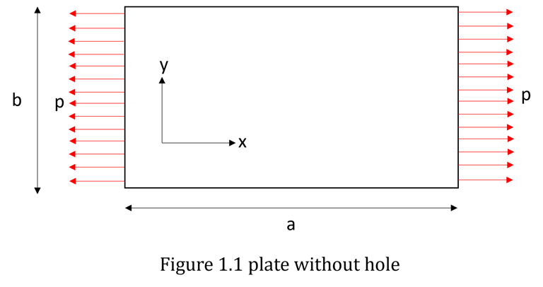
Consider a plane stress problem of finding stresses in a thin plate subjected to in plane loading as shown in figure 1.1 below. The principal dimensions of plate a and b are much greater than the thickness of plate. Since the problem is simple one, we can solve it using the simple analytical formulae. Now let us drill a hole of diameter Φ exactly at the center of plate. As shown in figure 1.2

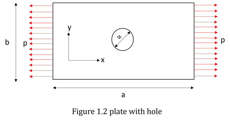
here due to curved boundary (circumference of circle) present in the domain, it is difficult to calculate the stresses in the vicinity of hole using analytical methods. Also, there will be effect of stress concentration near curved boundary. In FEM we model this problem by meshing it with quadrilateral elements as shown below in figure 1.3. The quadrilaterals used here have 4 nodes although 8 node quadrilaterals are suited best to model this problem, but at this moment, we will not discuss much about this aspect.

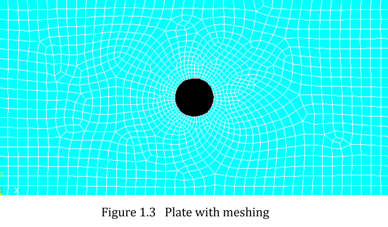
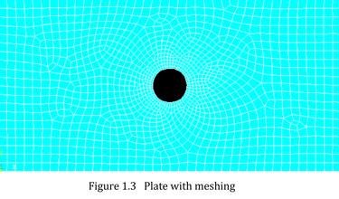
Now, the displacement which is the field variable in this problem which could assume infinite values in original problem shown in fig 1.2 can take only nodal values. By adopting the systematic process of FEM mentioned above, we can find stresses at various location in the plate. With the help of computers software, we can also show graphical distributions of stresses in a plate.

Comparison of FEM with analytical methods

• FEM offers far more advantages when compared with analytical methods. Below are some points worth noting when we compare FEM with analytical methods.

• In analytical methods exact equations are formed and solution obtained are also exact. However, on the other hand since FEM is a numerical method, it offers approximate solutions for exact equations.

• FEM easily takes into account complexities involved in geometry, forces and boundary conditions. On the other hand, analytical methods are of a little use when dealing with these practicalities and often these methods make over simplified assumptions to deal with such problems.

• Analytical methods are not suitable to deal with problems involving material discontinuities. On the other hand, FEM handles problems involving material discontinuities very well.

• When material is not isotropic, it becomes difficult to analyze problems using analytical methods. Whereas problems involving anisotropy and orthotropy can be easily dealt with FEM and results obtained are reasonably accurate.

• FEM handles non-linear analysis problems much easily without any difficulty.

Need of studying FEM

There has been always a debate about can we use commercially available FEA packages before learning fundamentals of Finite Element Method? Well, the answer to this question is yes one can do so but should not do it. Getting results from FEA packages is relatively simple but interpretation of these results to draw a conclusion is the most important concern for an engineer. Without having sound knowledge of FEM, one may not be able to answer following questions.

1. What type of element is to be used for meshing?

2. Whether the meshing is done properly or requires additional considerations?

3. How to incorporate proper boundary conditions?

4. Can given three-dimensional problem be analyzed as two-dimensional problem? (Which is often a case in stress analysis)

5. What are the limitations of element properties and how they affect accuracy of solution?

6. What are considerations in writing codes for pre-processors and post-processors for FEA packages?

Role of modern computers in implementation of FEM

The real potential of FEM came into picture after the advancements in new generation computers. With the developments in computer graphics and powerful image rendering capabilities available today as a result of evolution of powerful processors, GPU’s and faster RAMs, modern FEA packages are equipped with highly customized and user-friendly GUI. Also, it has benefited the graphical result post processing capabilities of FEA software. With the advancement in CAD/CAM, it is possible to export CAD models directly to the pre-processor of FEA software. Modern processors equipped with large memory makes it possible to solve the problems involving several thousands of nodes quickly and without any difficulty. Computers have made it possible to write computer programs and develop software’s built on FEM for dedicated applications like vehicle dynamics, acoustic analysis, multi DOF vibration problems, nonlinear analysis and may others.

Areas of application of FEM

A brief list of applications of FEM is given below. The actual list is far greater than this.

1. Manufacturing Industries: - Stress and thermal analysis of various parts such as pipes carrying hot fluids, pressure vessels, valves, molds, parts of hydraulic and pneumatic machineries subjected to high pressure and other similar applications.

2. Automotive industries: - Analysis of various engine parts like crankshaft, axles, flywheel, piston, cylinder, cylinder heads connecting rods, Crash analysis of vehicle body etc.

3. Analysis of heavy structures: - Seismic analysis of dams, tall towers and buildings etc.

4. Aircraft industry: - Crash analysis and aircraft, effect of wind stresses on wings and other parts of aircraft body etc.

5. Other applications: - Vibration and Acoustic problems, Fluid flow problems, seepage problems, Electromagnetic analysis of electronic components like transistors etc.

Final Thought

In this article, we have seen the brief overview of FEM. The process offers many advantages over the analytical methods. Its converts complex governing differential equation of problem into number of algebraic equations which are relatively easy to solve. In fact, FEM is a technique to numerically integrate a differential equation. The process is highly systematic and easy to automate due to which it can be easily coded in computer programs and further these programs can be used to create custom FEA software. The reason of popularity of FEM is that apart from its ready computer implementation, it gives fairly accurate results for those problems which are impossible to solve using analytical methods and even other numerical methods like Finite Difference method.

Leave a reply